Case study: a small manufacturer starts with a definition of normal, not a large model
Staff Jersey is an Italian knitted-fabric manufacturer with 10–49 employees and turnover of about €6.5 million. In a project with the ER2Digit European Digital Innovation Hub and Centro Qualità Tessile, the company tested automated detection of defects in moving fabric. The official case page was published on 14 October 2025.
The problem is familiar to many small manufacturers: an operator performs monotonous visual inspection while the product mix changes faster than a labelled dataset can grow. A stain, tear, or pattern irregularity may be rare, but missing it can cause scrap, rework, and a customer claim. A conventional vision project soon runs out of real examples of every defect type.
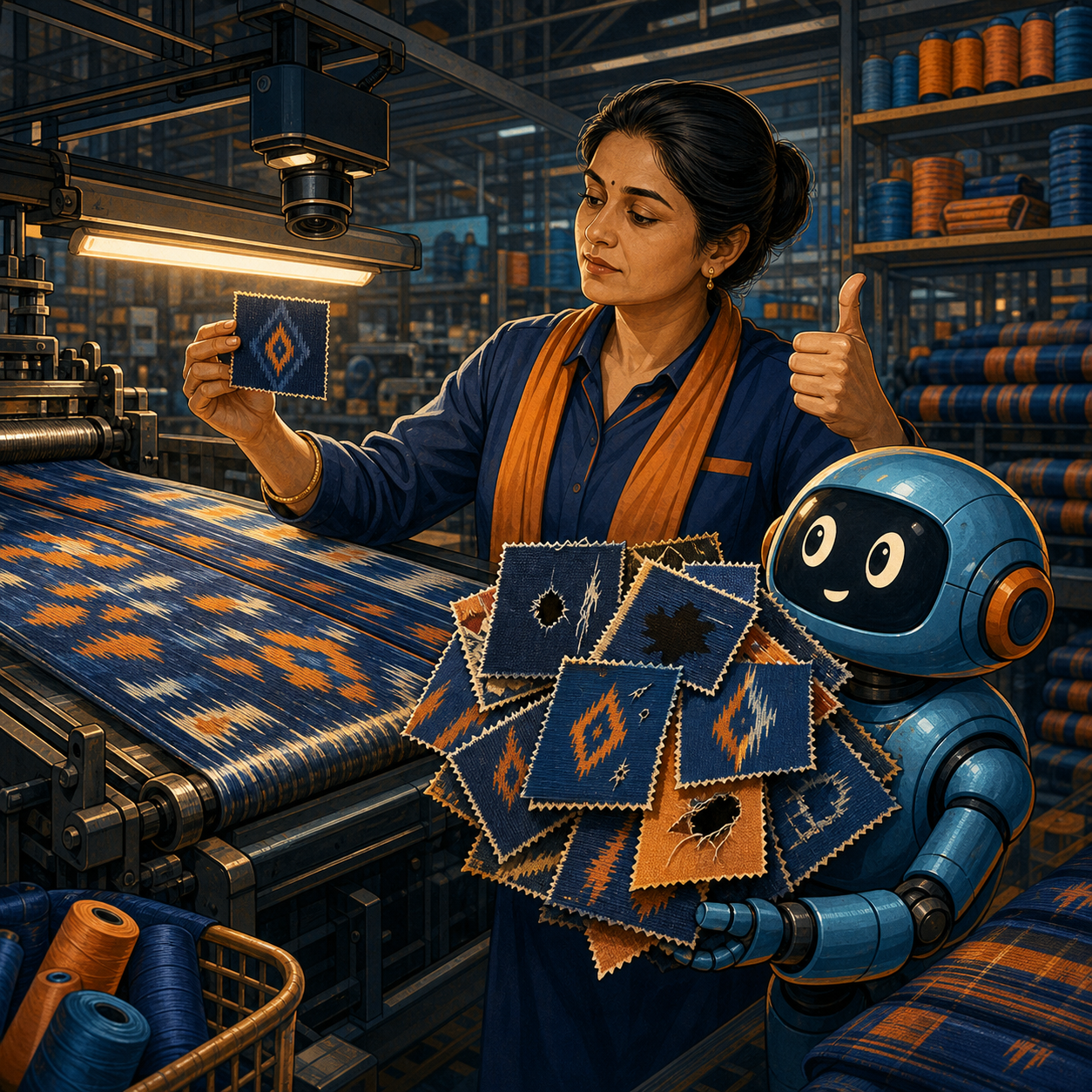
The pilot used two practical ideas. First, the operator confirms a clean section of each new fabric, which becomes the current reference for “normal.” Second, semi-synthetic defects and their segmentation masks are generated from compliant fabric images. The model can therefore learn to localise anomalies without a person drawing a pixel mask around every simulated hole or stain.
What was installed on the shop floor
The official description provides unusually practical acquisition details. A GoPro HERO13 Black with a macro lens and remote control was mounted near the machine. The camera was attached to a grounded structural element, and the existing lamp was aligned to reduce shadows. Fabric moved through the field of view, while time-lapse images were captured automatically every five seconds.
Ultra-high-resolution images were processed with sliding windows at multiple scales. The model produced a pixel-level anomaly map from 0 to 1. The 97.5th percentile of those values became the score for each crop: a single noisy pixel should not dominate the result, while a meaningful local anomaly should still increase the score.
The operational system has four engineering components:
- stable optics, illumination, and camera geometry;
- registration of the product, roll, pattern, line speed, and recipe change;
- a compliant reference confirmed by an operator;
- a model, a decision threshold, and a workflow for alerts.
Lamp glare, mount vibration, or a different knit scale can shift the input distribution more than a genuine anomaly.
Why a dynamic reference helps
For short production runs, a single class called “normal fabric” is too broad. Blue mélange, a thin plain knit, and a high-contrast pattern have different textures. Trying to place every variant into one fixed dataset turns the deployment into permanent labelling work.
A dynamic reference changes the task. After a changeover, the technologist confirms the first section as compliant. The system stores that reference with the batch parameters and detects deviations from the current production mode. This does not remove the need for a base model, but it narrows the gap between historical training data and the order currently running.
Reference confirmation must be a controlled action. The system must not silently learn that a defect at the beginning of a roll is normal. A safe process records:
- the responsible person or identifier;
- the reference image and confirmation time;
- its batch, product, and machine settings;
- a quick way to revoke an incorrect reference;
- an audit log of reference and model-version changes.
The human is not a fallback after AI fails. The human owns the definition of acceptable output for the current batch.
What synthetic defects solve—and what they do not
Surface-anomaly methods can be trained largely on defect-free images. The DRAEM research paper describes an approach in which simulated anomalies help a model reconstruct normal appearance and localise deviations. Semi-synthetic examples are particularly useful when real defects are scarce and pixel-level manual annotation is expensive.
Synthetic data quickly creates varied shapes and automatically supplies segmentation masks. However, a generator only reproduces the logic built into it. A real pulled thread, lubricant stain, wrinkle, or fabric flutter may look different. Synthetic data must stay out of the final holdout and cannot be the sole evidence of quality.
The blind test should contain real examples unseen during training. Neighbouring crops from the same roll must not be randomly split between training and testing: their background and structure are nearly identical, which can inflate the score. The correct split unit is a complete roll, batch, or production run.
How to interpret the reported 99.93%
The EDIH page describes a test of 200 unseen 256×256 crops: 100 normal and 100 real defective samples. The defective crops—tears, stains, and pattern irregularities—were manually selected. On this set, the reported AUROC was 99.93%, AUPRC was 99.93%, and accuracy at a 0.5 threshold was 99.50%.
These results show that the model almost perfectly separated the selected normal and defective crops in this small, balanced test. They do not answer the main production question.
AUROC and AUPRC evaluate ranking across possible thresholds. They do not choose the point at which a line should alert an operator. Accuracy on a dataset where defects account for 50% also cannot be transferred to a stream where defects may be fractions of a percent. On a real line, thousands of normal windows can create an operationally significant number of alerts even with high specificity.
Before deployment, the evaluation should include:
- recall for every economically critical defect type;
- false alerts per roll, hour, and thousand metres;
- delay between defect appearance and alert;
- the share of fabric width and length actually covered by the camera;
- separate results by material, pattern, speed, and shift;
- performance on entirely new rolls at natural defect prevalence.
The threshold must follow decision cost, not the appearance of an ROC curve. If one missed tear ruins a roll, recall dominates. If each false stop destabilises the machine and produces more waste, that cost must also shape the threshold.
A practical local architecture
This application does not require a large language model. A compact computer-vision model can run on an industrial computer or workstation near the line. High-resolution production images, recipes, and order details can remain inside the factory.
A practical system includes:
- a camera service that collects frames and checks exposure, focus, and missing captures;
- a batch registry containing the product, roll, speed, and active clean reference;
- local inference that tiles images, produces anomaly maps, and aggregates scores;
- rules that merge neighbouring anomalous windows into one event and suppress duplicates;
- a buffer that preserves frames before and after an alert;
- an operator interface to confirm, reject, or escalate the event;
- a quality log and reviewed dataset for the next model version;
- monitoring for alert frequency, lighting drift, and score-distribution shifts.
At first, the system should run in shadow mode and must not stop equipment. Automatic stopping is appropriate only after latency, fail-safe behaviour, and false-command cost have been verified. Highlighting a region and recommending inspection is a safer first stage.
Economics: count metres, not images
A model calculation should be tied to physical output. Suppose a line produces M metres per month, the contribution loss from an undetected defect is L per metre, and the pilot reduces affected length by a fraction R. The expected monthly avoided loss is M × defective-output share × L × R.
From that amount, subtract:
- camera, lighting, mount, and edge-compute costs;
- integration with batch identifiers and the quality log;
- technologist time for reference approval and alert review;
- losses caused by false stops;
- support, calibration, and retraining.
This is a model, not a return-on-investment promise. Before the pilot, the company should use its own three to six months of data: rework, scrap, claims, manual-inspection time, and stop cost. If those numbers do not exist, the project must improve quality accounting before it can prove AI value.
A 30-day pilot without an expensive integration
The first month can run without any command to stop the line.
1. Select three to five fabric families, 20–30 rolls, and two or three economically important defects.
2. Fix the camera, light, capture rate, and roll identifier; measure blind areas at different speeds.
3. Collect clean references and real defects. Split training and validation by complete roll.
4. Add synthetic anomalies only to training and preserve their provenance.
5. Run in shadow mode. Operators continue the normal process, while model scores do not influence decisions.
6. Compare events after each shift: misses, false alerts per roll, latency, and confirmation time.
7. Tune the threshold using the monetary cost of errors and repeat the test on new batches.
Pilot success means an agreed ceiling for critical misses, acceptable alert load, required coverage, and a credible payback period. Even a failed test can show whether the bottleneck is optics, reference management, data, or the model.
What a manager should take away
The Staff Jersey case offers a realistic path for small manufacturers: stabilise acquisition, give the technologist control over the definition of normal, use synthetic defects to bootstrap learning, and validate on entirely new real rolls.
The next step is not a complex platform purchase. Choose one line, 20–30 rolls, and one month of shadow testing. Measure defects and false alerts per unit of output, then choose the threshold from the cost of errors. That is how an impressive metric becomes an operational investment decision.