Bottom line
A local model can be economical with stable demand, restrictions on transferring data, or several workloads sharing one server. But comparing “GPU price versus API bill” leaves out operations, redundancy, staff time, and answer quality. Calculate the cost of an accepted result at a defined response time and availability level.
Test the idea in two or three weeks: collect actual demand, compare identical requests in the cloud and on a target local node, and estimate a break-even range. All figures below are model assumptions, not market prices.
Build a complete cost model
Cloud API costs usually vary with input and output tokens. Also include retries, long contexts, peaks, paid features, document transfer, minimum charges, and a fallback route. Use logs from ordinary weeks, not the busiest day or a five-prompt demo.
Break local costs into four groups:
- **Hardware:** server, accelerator, memory, disks, networking, UPS, and hosting. Spread the one-time price over the assumed useful life; that is an assumption, not a service-life guarantee.
- **Power and cooling:** measured average node power, operating hours, tariff, and room infrastructure. Nameplate peak power is not average consumption.
- **Operations:** monitoring, updates, backups, access, incidents, version testing, and user support. Salaried staff time still has a cost.
- **Quality and risk:** share of answers corrected by a person, latency, outages, model license, and cost of error. An answer an employee rewrites is not cheap.
Include launch work: data preparation, model configuration, integration, secure deployment, and a test set. Account for it separately or allocate it monthly, but do not treat it as zero just because it was paid once.
Measure the workload
For four ordinary weeks, count requests, input and output length, time of day, latency, retries, and the share accepted without edits. Remove personal data or measure inside an approved environment. Separate tasks—document search, email drafts, field extraction, classification—because their quality criteria may differ.
Build a test set from real, de-identified examples. Agree on reference answers or evaluation criteria with the process owner. Compare the same prompts, context, and knowledge-base version. Measure not only generation speed, but time to the first useful answer, end-to-end time, errors, refusals, and follow-on human work.
For a local server, compare these results with telemetry from the same period. NVIDIA DCGM documents GPU power and energy metrics; vLLM exposes per-request metrics, including processing time and token throughput. Tie them to a test task to estimate energy per accepted answer. Documentation does not guarantee a metric is available on a specific card, driver, and build; verify it on the target node.
A break-even example
Assume, for illustration, 12,000 requests per month, each averaging 2,000 input and 500 output tokens: 24 million input and 6 million output tokens. With API rates per million tokens, variable cost is 24 times the input price plus 6 times the output price. Add minimum charges, fallback, and human review. Use your contract and logs for a real decision.
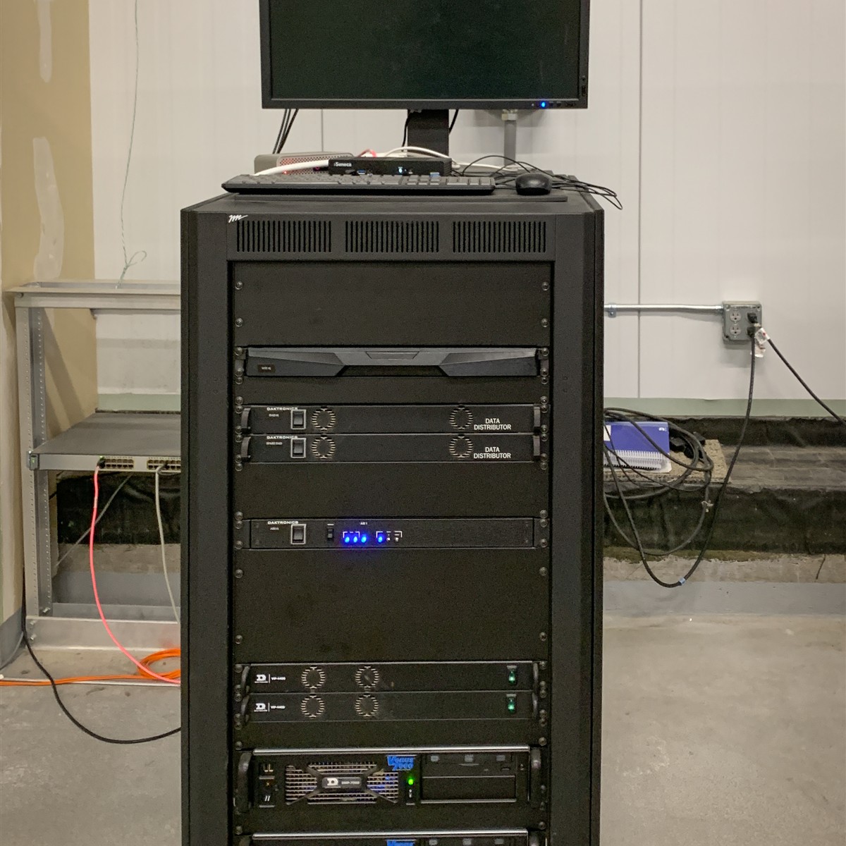
A hypothetical local node costing RUB 600,000 and amortized over 36 months costs RUB 16,667 monthly. If the whole server averages 0.8 kW around the clock, it uses 576 kWh in 30 days. An illustrative 1.3 factor for cooling and losses brings this to about 749 kWh; at a model tariff of RUB 10 per kWh, power costs RUB 7,490. Add 12 operations hours at RUB 1,500 (RUB 18,000) and RUB 4,000 for support: about RUB 46,200 per month.
This does not prove local deployment is cheaper. Taxes, cost of capital, initial integration, a backup node, and outages are excluded. If availability needs two servers, include both. If the node also runs search or speech recognition, allocate costs across workloads only if they actually use it.
In this scenario, local deployment begins to win on direct costs when a comparable cloud option exceeds about RUB 46,200 monthly. But quality, latency, security, and availability must be comparable. More local-model errors increase review time and the break-even point. Idle time raises cost per request; seasonal peaks can be hidden by an annual average.
Run a short pilot
1. **Choose a task and owner.** Define an accepted result, response-time limit, and who handles exceptions. Start with a business criterion, not a model.
2. **Record a baseline.** Capture volume, API spend, staff time, and correction rates over ordinary weeks; mark seasonality separately.
3. **Compare options.** Run cloud and local tests on the same de-identified examples under the same evaluation rules.
4. **Collect metrics.** Track energy, utilization, latency, throughput, retries, outages, and minutes of human review; separate test from background load.
5. **Check operations.** Review the license, updates, access, backups, and failover plan. Hosting “inside” does not itself ensure security or compliance.
6. **Calculate three scenarios.** Normal, peak, and low season; include downtime and fallback. Compare an annual range, not one figure.
Human review should not be removed from the economics. NIST’s generative AI profile warns about excessive trust in machine outputs and recommends tailoring oversight and testing to the scenario. Sampling may be enough for an internal instruction draft; a customer reply, accounting entry, or order change needs stricter automation boundaries.
Mistakes that distort the result
- Pricing API use from a marketing table while ignoring context, retries, and fallback.
- Using rated power instead of measurements, or forgetting cooling and losses.
- Stretching amortization and ignoring repairs, accelerator refresh, and residual value.
- Comparing different models or judging quality from a few successful examples.
- Excluding administration, incidents, and employee review time.
- Naming a winner without pricing errors, latency, and unavailability.
Uptime Institute includes electricity, cooling, equipment maintenance, and staff in data-center operating expenses. An office node is smaller, but the principle is the same: electricity is not the whole TCO. Its overview is a useful category checklist, though large-facility averages should not be transferred directly to an SMB server.
A decision for the manager
Ask the team for four numbers per option: monthly cost, cost per accepted result, share corrected by a person, and availability at peak hours. Show assumptions and a range. If local deployment is cheaper only at full utilization, check whether that utilization exists. If the API costs more but needs no on-call engineer or second server, include that difference.
Next, select one internal process, export a de-identified week of usage, and request two estimates: API cost at actual volume and a local pilot with power measurements. Then decide whether to buy a server, rent compute, or keep the model in an API. The pilot should not prove a preselected architecture; it should quickly reveal full cost and limitations.
This is a model calculation: RUB 600,000, 36 months, 0.8 kW, a 1.3 factor, RUB 10 per kWh, 12 hours at RUB 1,500, and RUB 4,000 for support are illustrative assumptions, not quotes or a hardware recommendation.