What 24 Vision Actually Validated
24 Vision is a small Czech machine-vision company with 10–49 employees, according to the European Digital Innovation Hubs case record. The company wanted to move from rule-based checks such as “if contrast exceeds a threshold, flag a defect” toward machine-learning-based defect classification. Its first obstacle, however, was more fundamental: it had neither a representative image dataset nor validated evidence showing which optical configuration could reveal defects consistently across different materials, finishes and colours.
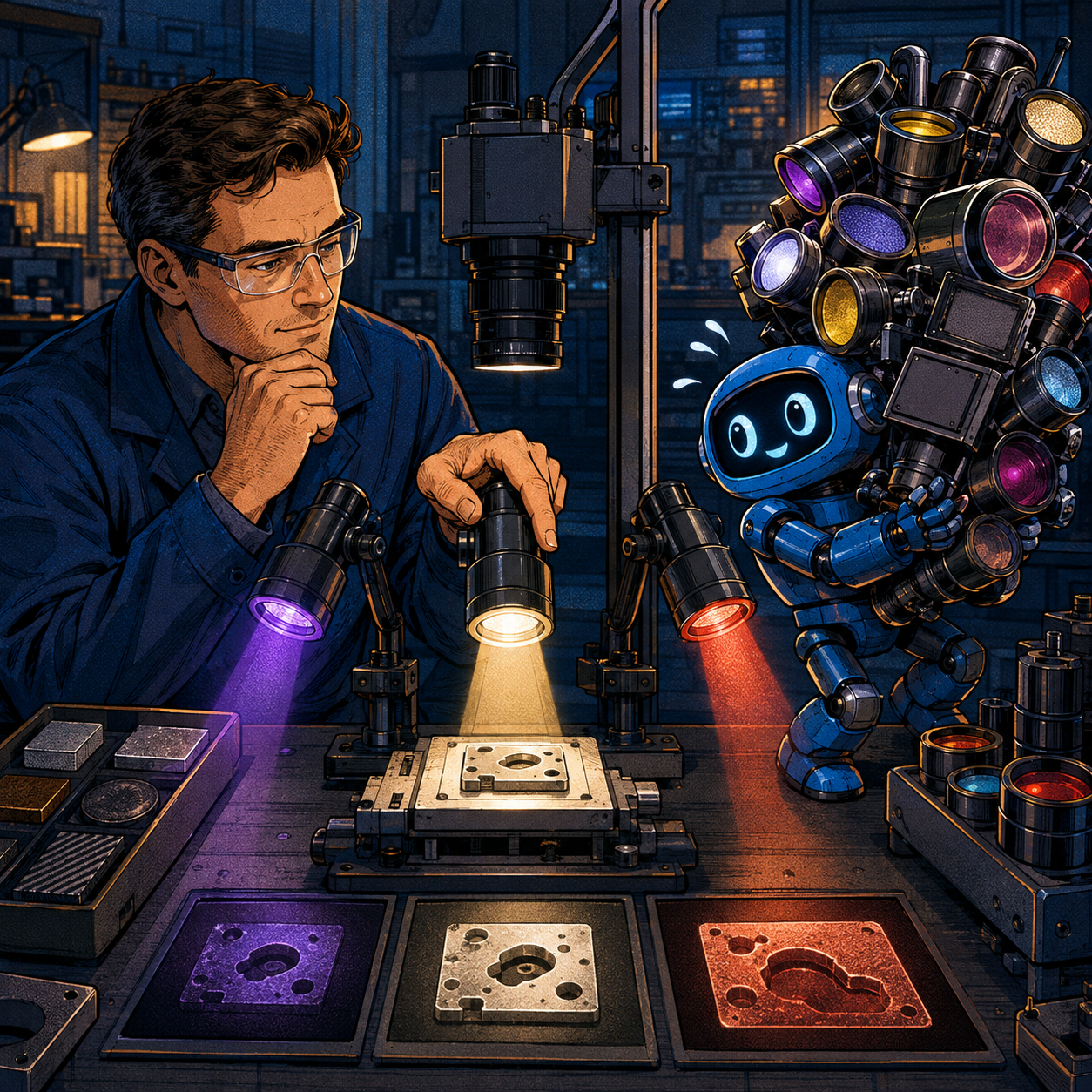
Together with EDIH-DIGIMAT, the company ran a Test Before Invest engagement: a laboratory validation before buying and building a production system. The team varied sample holders, camera position, a polarising filter, lighting geometry and spectral range. Ultraviolet, visible and near-infrared configurations were compared.
For the submitted samples, only the visible range consistently highlighted defects across all surface types. The team produced a structured dataset and a documented imaging method. The theoretical error below one pixel reported by the case describes the optical and geometric measurement chain; it is not classifier accuracy and does not prove production readiness.
That distinction matters. The public case documents a completed validation of the data-acquisition method, but it does not report production metrics such as defect escape rate, false rejection, cycle time, resilience to new batches or savings per unit. The useful conclusion is therefore not “AI replaced quality control.” It is that the company removed an early technical risk before committing capital to models and equipment.
Why the Model Starts with Lighting
A visual-inspection system has five connected layers:
- the quality standard: which defect is critical and who resolves borderline cases;
- the optical scene: lighting, camera, lens, filters, distance and part fixation;
- the data: images, annotations, product version and capture conditions;
- the model: detection, segmentation or classification;
- the production decision: accept the item, route it for review or stop the process.
If a defect barely differs from the background, the model learns noise. It may look accurate on a randomly split dataset and then fail after a lamp is replaced, the material supplier changes or a part is rotated. Independent reviews of industrial machine vision similarly note that surface properties and environmental conditions affect detection, while real deployment must be tested against changes in lighting, cameras, products and rare defect types.
A sound pilot therefore does not begin with the largest neural network. It begins by making the defect visible, repeatable and measurable. That exercise may reveal that a deterministic algorithm is sufficient. When defect appearance is genuinely variable, it provides a justified reason to use a learned model.
How a Small Manufacturer Can Reuse the Approach
For an SME, a two-environment architecture is practical.
The first environment is a laboratory. Samples are captured under several configurations, and a quality engineer or process specialist confirms the labels. Speed matters less here than the ability to change lighting and mechanics quickly while recording each setup as a versioned experiment.
The second environment is production. Once the optical design is chosen, the camera and lighting are shielded from ambient light, exposure is locked, and a reference sample is used to check drift regularly. The model can run locally on an industrial PC or an on-premises server: images remain inside the company, latency is predictable, and the line does not depend on an external API. Local deployment does not solve quality by itself; monitoring, decision logs and a safe failure mode are still required.
The data flow is straightforward:
- a line trigger links each frame to an item or batch;
- the capture service stores the image and camera parameters;
- the model returns the defect class, location and confidence;
- a business rule compares the result with the approved threshold;
- borderline cases go to an operator instead of directly to scrap;
- the confirmed decision is written to MES, ERP or the quality log;
- new errors enter the dataset only after human review.
An agent is unnecessary in the first version. A short, inspectable pipeline with explicit states is more valuable. An LLM may later help draft explanations or shift reports, but it should not replace the measurement model or the line-stop rule.
What Data to Collect Before Training
The minimum package starts with a defect register. Each type needs an image, acceptable and unacceptable examples, minimum size, cost of error and a named decision owner. Then the team needs a variation matrix covering material, colour, finish, supplier, machine, shift, part position and lighting condition.
The dataset must contain more than clean laboratory defects. It also needs good parts, contamination, glare, transport scratches and borderline examples. Training and validation data should be split by batch or date, not randomly across adjacent frames; otherwise near-duplicate images can land on both sides and inflate the estimate.
Capture metadata and the optical-configuration version must be stored separately. Changing the light, lens or distance creates a new input-data version. Without that discipline, the team cannot tell whether the model deteriorated or the scene changed.
Economics: Measure Accepted Decisions, Not Accuracy
The 24 Vision case does not disclose the budget or payback period. Its economic logic is avoided premature capital expenditure: the specialist optical laboratory was used during selection, but the company did not first have to purchase every equipment option.
For an internal pilot, a useful unit metric is:
`cost per accepted inspection = (test rig depreciation + compute + labelling + rechecks + downtime) / decisions confirmed by quality staff`.
A model calculation might assume one operation, two critical defect classes and three common product variants. Those are planning assumptions, not 24 Vision results. The team first estimates the current cost of manual inspection, false rejection and escapes. It then runs the system in shadow mode against human inspection without affecting product release.
Automatic action is justified only when the upper risk bound for escapes is acceptable, false rejection does not consume the benefit, and latency fits the line takt time. Otherwise the pilot may be technically interesting but economically useless.
Limitations and Risks
The primary risk is the move from laboratory to shop floor. Vibration, dust, reflections, heat, light-source ageing and new material batches create data shift. A result on one sample set cannot be generalised automatically to another product.
The second risk is rare defects. A large collection of normal images does not replace enough confirmed high-severity cases. Those cases require conservative thresholds and a human-review path.
The third risk is confusing measurement precision with decision quality. Sub-pixel rig error says nothing about defect escape rate. Before production rollout, the team must separately measure recall for critical classes, false rejection, operator-review rate, latency and batch-level stability.
Finally, the laboratory conclusion about visible light applies to the tested samples. A new material or finish may require UV, VIS and NIR comparison again. The value of the method is that the validation can be repeated, not that one spectrum has been declared universal.
A Practical Next Step
In ten working days, a manufacturer can test the hypothesis without buying a complete inspection line:
1. Select one operation and one costly failure mode.
2. Agree on the defect standard and the manual confirmation rule.
3. Collect real samples from several batches.
4. Capture them under two or three lighting options with fixed geometry.
5. Measure contrast and repeatability before training a model.
6. If the scene is stable, label a pilot set and validate by separate batches.
7. Run in shadow mode and calculate the cost per confirmed decision.
If the defect is unstable after step 5, change the optics or capture method rather than the model. That is the central lesson of this case: the cheapest neural network is the one you do not train on poorly visible data.